Benchmarking Message Queue Latency

About a year and a half ago, I published Dissecting Message Queues, which broke down a few different messaging systems and did some performance benchmarking. It was a naive attempt and had a lot of problems, but it was also my first time doing any kind of system benchmarking. It turns out benchmarking systems correctly is actually pretty difficult and many folks get it wrong. I don’t claim to have gotten it right, but over the past year and a half I’ve learned a lot, tried to build some better tools, and improve my methodology.

Tooling and Methodology

The Dissecting Message Queues benchmarks used a framework I wrote which published a specified number of messages effectively as fast as possible, received them, and recorded the end-to-end latency. There are several problems with this. First, load generation and consumption run on the same machine. Second, the system under test runs on the same machine as the benchmark client—both of these confound measurements. Third, running “pedal to the metal” and looking at the resulting latency isn’t a very useful benchmark because it’s not representative of a production environment (as Gil Tene likes to say, this is like driving your car as fast as possible, crashing it into a pole, and looking at the shape of the bumper afterwards—it’s always going to look bad). Lastly, the benchmark recorded average latency, which, for all intents and purposes, is a useless metric to look at.

I wrote Flotilla to automate “scaled-up” benchmarking—running the broker and benchmark clients on separate, distributed VMs. Flotilla also attempted to capture a better view of latency by looking at the latency distribution, though it only went up to the 99th percentile, which can sweep a lot of really bad things under the rug as we’ll see later. However, it still ran tests at full throttle, which isn’t great.

Bench is an attempt to get back to basics. It’s a simple, generic benchmarking library for measuring latency. It provides a straightforward Requester interface which can be implemented for various systems under test. Bench works by attempting to issue a fixed rate of requests per second and measuring the latency of each request issued synchronously. Latencies are captured using HDR Histogram, which observes the complete latency distribution and allows us to look, for example, at “six nines” latency.

Introducing a request schedule allows us to measure latency for different configurations of request rate and message size, but in a “closed-loop” test, it creates another problem called coordinated omission. The problem with a lot of benchmarks is that they end up measuring service time rather than response time, but the latter is likely what you care about because it’s what your users experience.

The best way to describe service time vs. response time is to think of a cash register. The cashier might be able to ring up a customer in under 30 seconds 99% of the time, but 1% of the time it takes three minutes. The time it takes to ring up a customer is the service time, while the response time consists of the service time plus the time the customer waited in line. Thus, the response time is dependent upon the variation in both service time and the rate of arrival. When we measure latency, we really want to measure response time.

Now, let’s think about how most latency benchmarks work. They usually do this:

1. Note timestamp before request, t₀.
2. Make synchronous request.
3. Note timestamp after request, t₁.
4. Record latency t₁ – t₀.
5. Repeat as needed for request schedule.

What’s the problem with this? Nothing, as long as our requests fit within the specified request schedule.  For example, if we’re issuing 100 requests per second and each request takes 10 ms to complete, we’re good. However, if one request takes 100 ms to complete, that means we issued only one request during those 100 ms when, according to our schedule, we should have issued 10 requests in that window. Nine other requests should have been issued, but the benchmark effectively coordinated with the system under test by backing off. In reality, those nine requests waited in line—one for 100 ms, one for 90 ms, one for 80 ms, etc. Most benchmarks don’t capture this time spent waiting in line, yet it can have a dramatic effect on the results. The graph below shows the same benchmark with coordinated omission both uncorrected (red) and corrected (blue):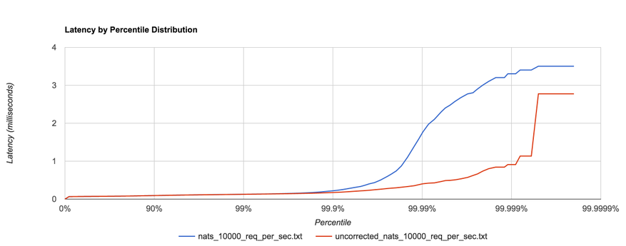

HDR Histogram attempts to correct coordinated omission by filling in additional samples when a request falls outside of its expected interval. We can also deal with coordinated omission by simply avoiding it altogether—always issue requests according to the schedule.

Message Queue Benchmarks

I benchmarked several messaging systems using bench—RabbitMQ (3.6.0), Kafka (0.8.2.2 and 0.9.0.0), Redis (2.8.4) pub/sub, and NATS (0.7.3). In this context, a “request” consists of publishing a message to the server and waiting for a response (i.e. a roundtrip). We attempt to issue requests at a fixed rate and correct for coordinated omission, then plot the complete latency distribution all the way up to the 99.9999th percentile. We repeat this for several configurations of request rate and request size. It’s also important to note that each message going to and coming back from the server are of the specified size, i.e. the “response” is the same size as the “request.”

The configurations used are listed below. Each configuration is run for a sustained 30 seconds.

• 256B requests at 3,000 requests/sec (768 KB/s)
• 1KB requests at 3,000 requests/sec (3 MB/s)
• 5KB requests at 2,000 requests/sec (10 MB/s)
• 1KB requests at 20,000 requests/sec (20.48 MB/s)
• 1MB requests at 100 requests/sec (100 MB/s)

These message sizes are mostly arbitrary, and there might be a better way to go about this. Though I think it’s worth pointing out that the Ethernet MTU is 1500 bytes, so accounting for headers, the maximum amount of data you’ll get in a single TCP packet will likely be between 1400 and 1500 bytes.

The system under test and benchmarking client are on two different m4.xlarge EC2 instances (2.4 GHz Intel Xeon Haswell, 16GB RAM) with enhanced networking enabled.

Redis and NATS

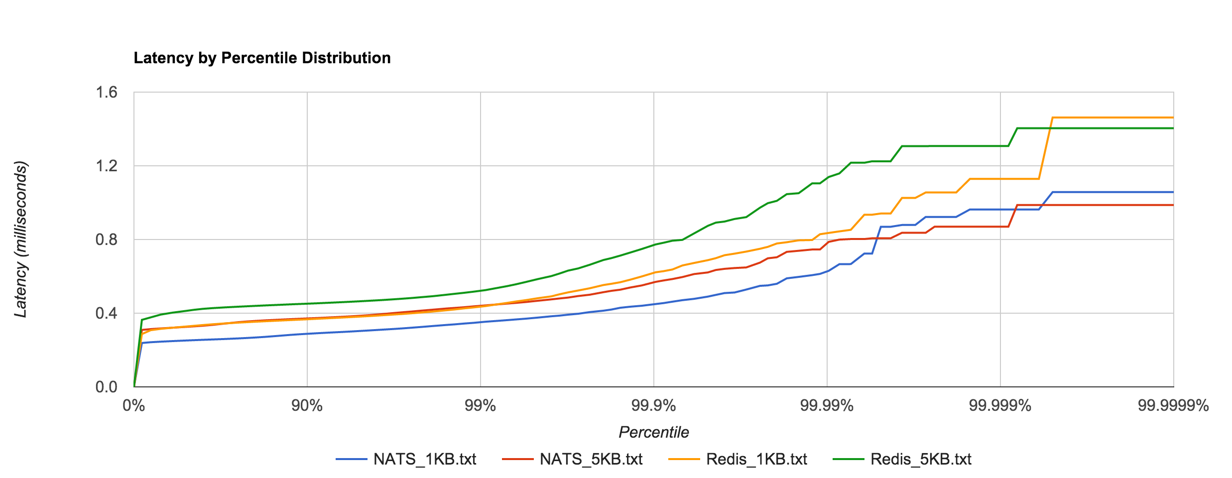
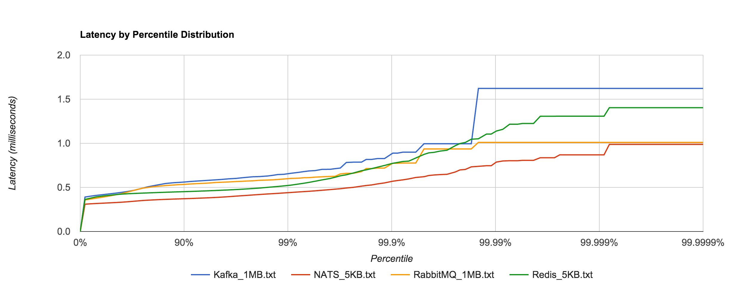
Redis pub/sub and NATS have similar performance characteristics. Both offer very lightweight, non-transactional messaging with no persistence options (discounting Redis’ RDB and AOF persistence, which don’t apply to pub/sub), and both support some level of topic pattern matching. I’m hesitant to call either a “message queue” in the traditional sense, so I usually just refer to them as message brokers or buses. Because of their ephemeral nature, both are a nice choice for low-latency, lossy messaging.

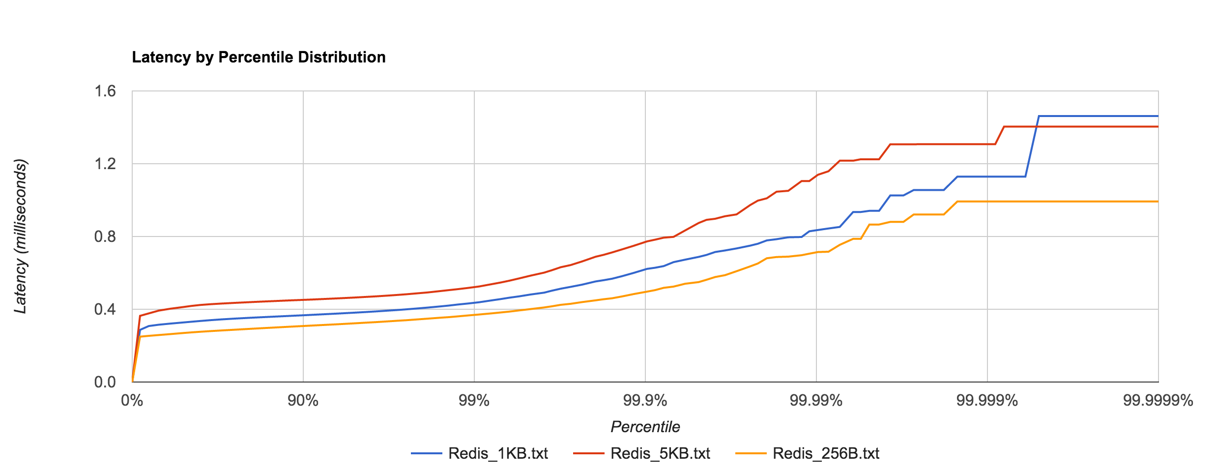
Redis tail latency peaks around 1.5 ms.

NATS performance looks comparable to Redis. Latency peaks around 1.2 ms.

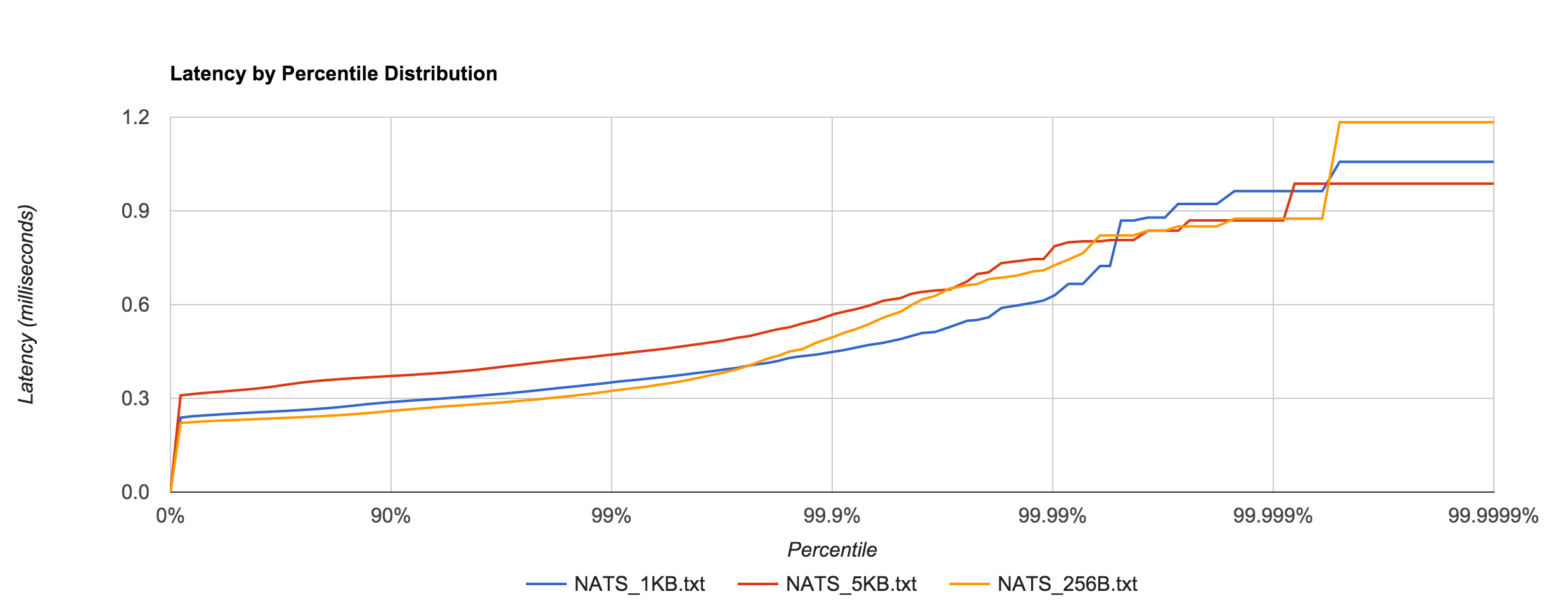
The resemblance becomes more apparent when we overlay the two distributions for the 1KB and 5KB runs. NATS tends to be about 0.1 to 0.4 ms faster.

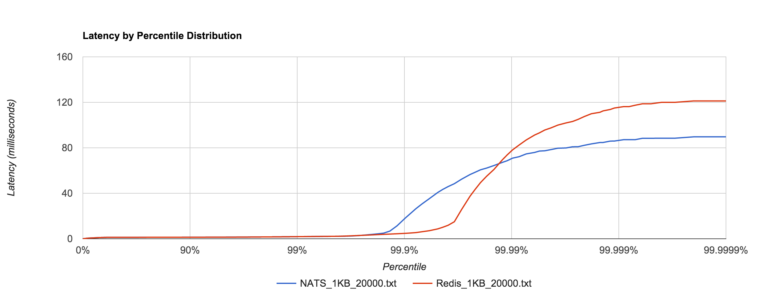
The 1KB, 20,000 requests/sec run uses 25 concurrent connections. With concurrent load, tail latencies jump up, peaking around 90 and 120 ms at the 99.9999th percentile in NATS and Redis, respectively.

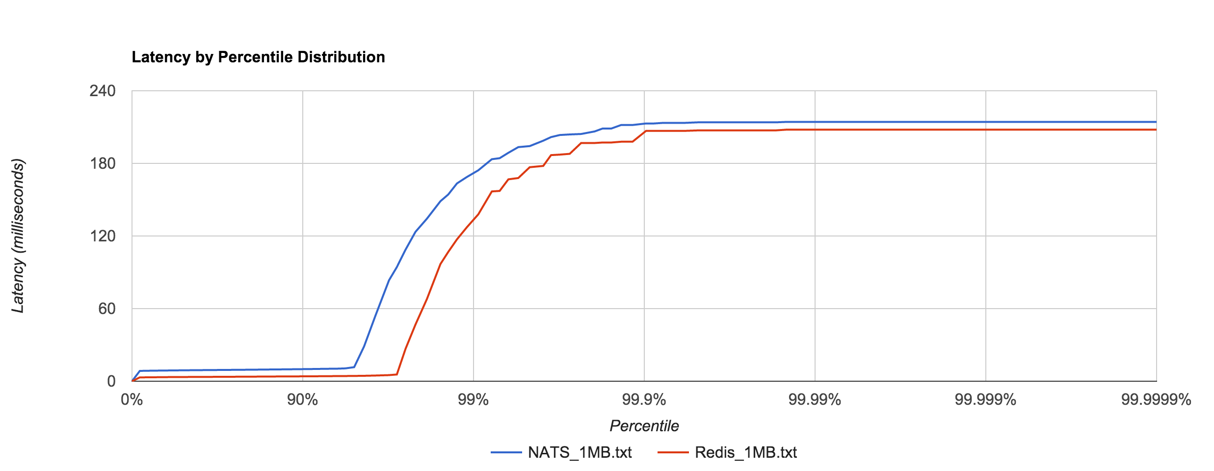
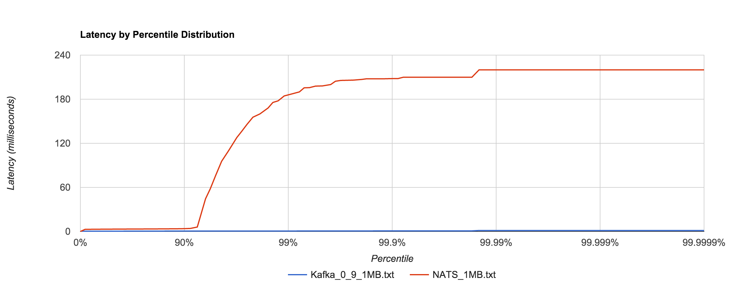
Large messages (1MB) don’t hold up nearly as well, exhibiting large tail latencies starting around the 95th and 97th percentiles in NATS and Redis, respectively. 1MB is the default maximum message size in NATS. The latency peaks around 214 ms. Again, keep in mind these are synchronous, roundtrip latencies.

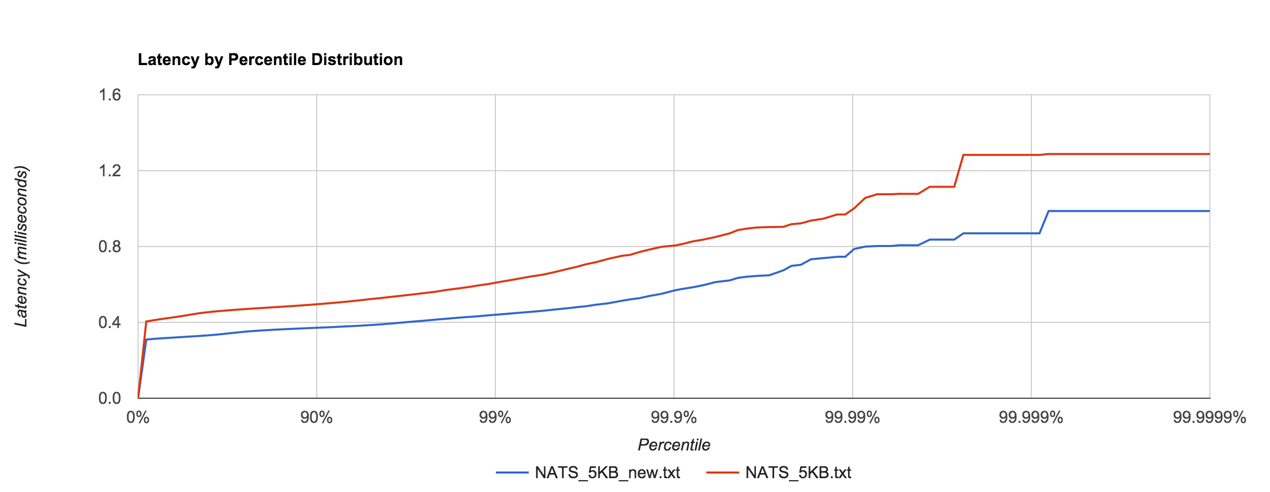
Apcera’s Ivan Kozlovic pointed out that the version of the NATS client I was using didn’t include a recent performance optimization. Before, the protocol parser scanned over each byte in the payload, but the newer version skips to the end (the previous benchmarks were updated to use the newer version). The optimization does have a noticeable effect, illustrated below. There was about a 30% improvement with the 5KB latencies.

The difference is even more pronounced in the 1MB case, which has roughly a 90% improvement up to the 90th percentile. The linear scale in the graph below hides this fact, but at the 90th percentile, for example, the pre-optimization latency is 10 ms and the optimized latency is 3.8 ms. Clearly, the large tail is mostly unaffected, however.

In general, this shows that NATS and Redis are better suited to smaller messages (well below 1MB), in which latency tends to be sub-millisecond up to four nines.

RabbitMQ and Kafka

RabbitMQ is a popular AMQP implementation. Unlike NATS, it’s a more traditional message queue in the sense that it supports binding queues and transactional-delivery semantics. Consequently, RabbitMQ is a more “heavyweight” queuing solution and tends to pay an additional premium with latency. In this benchmark, non-durable queues were used. As a result, we should see reduced latencies since we aren’t going to disk.

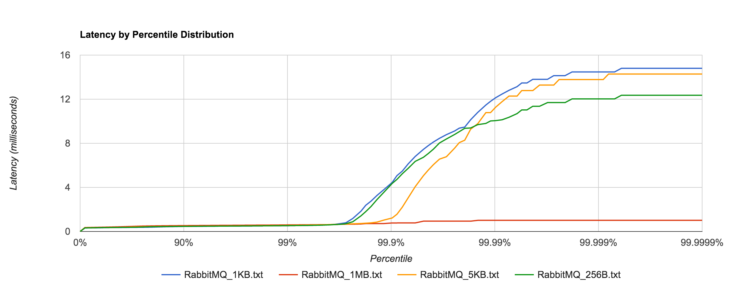
Latency tends to be sub-millisecond up to the 99.7th percentile, but we can see that it doesn’t hold up to NATS beyond that point for the 1KB and 5KB payloads.

Kafka, on the other hand, requires disk persistence, but this doesn’t have a dramatic effect on latency until we look at the 94th percentile and beyond, when compared to RabbitMQ. Writes should be to page cache with flushes to disk happening asynchronously. The graphs below are for 0.8.2.2.

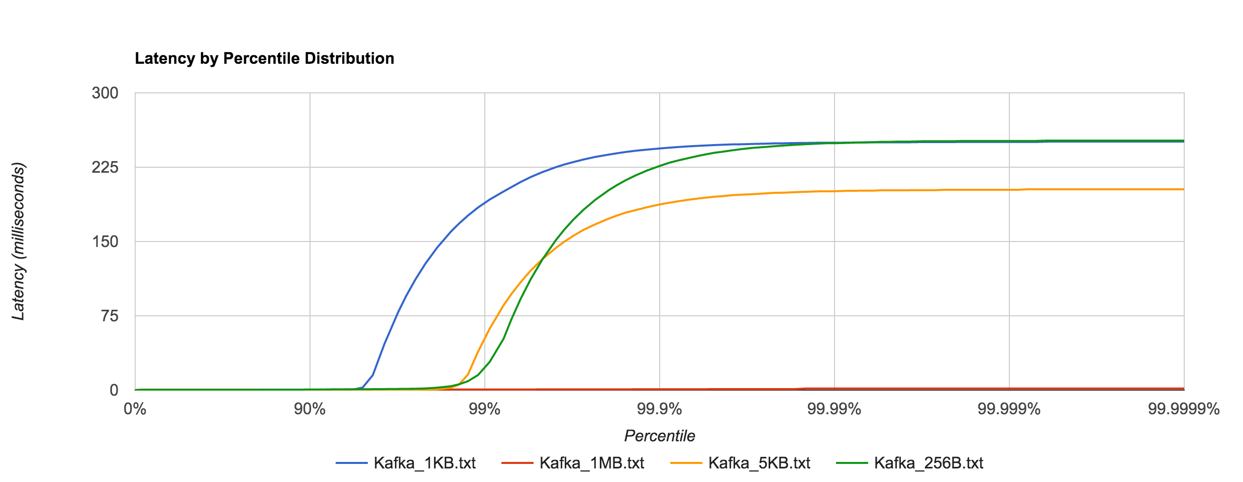
Once again, the 1KB, 20,000 requests/sec run is distributed across 25 concurrent connections. With RabbitMQ, we see the dramatic increase in tail latencies as we did with Redis and NATS. The RabbitMQ latencies in the concurrent case stay in line with the previous latencies up to about the 99th percentile. Interestingly, Kafka, doesn’t appear to be significantly affected. The latencies of 20,000 requests/sec at 1KB per request are not terribly different than the latencies of 3,000 requests/sec at 1KB per request, both peaking around 250 ms.

What’s particularly interesting is the behavior of 1MB messages vs. the rest. With RabbitMQ, there’s almost a 14x difference in max latencies between the 5KB and 1MB runs with 1MB being the faster. With Kafka 0.8.2.2, the difference is over 126x in the same direction. We can plot the 1MB latencies for RabbitMQ and Kafka since it’s difficult to discern them with a linear scale.

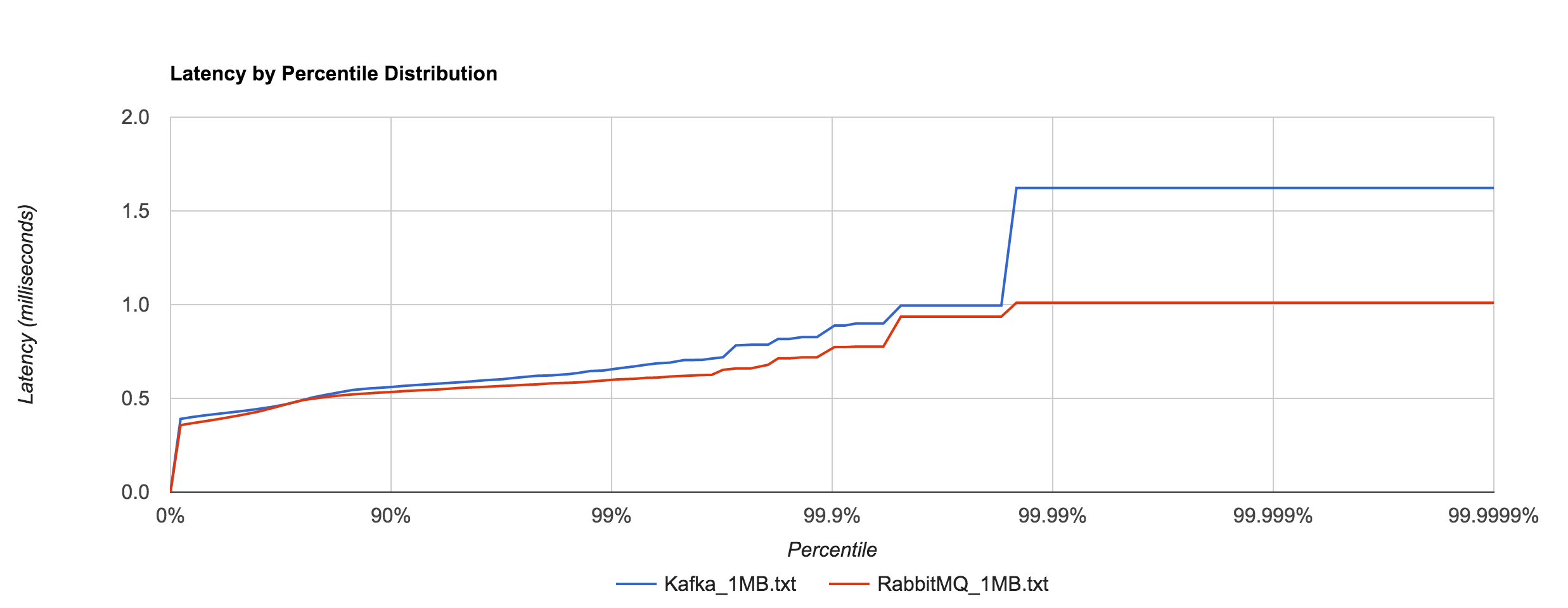
I tried to understand what was causing this behavior. I’ve yet to find a reasonable explanation for RabbitMQ. Intuition tells me it’s a result of buffering—either at the OS level or elsewhere—and the large messages cause more frequent flushing. Remember that these benchmarks were with transient publishes. There should be no disk accesses occurring, though my knowledge of Rabbit’s internals are admittedly limited. The fact that this behavior occurs in RabbitMQ and not Redis or NATS seems odd. Nagle’s algorithm is disabled in all of the benchmarks (TCP_NODELAY). After inspecting packets with Wireshark, it doesn’t appear to be a problem with delayed acks.

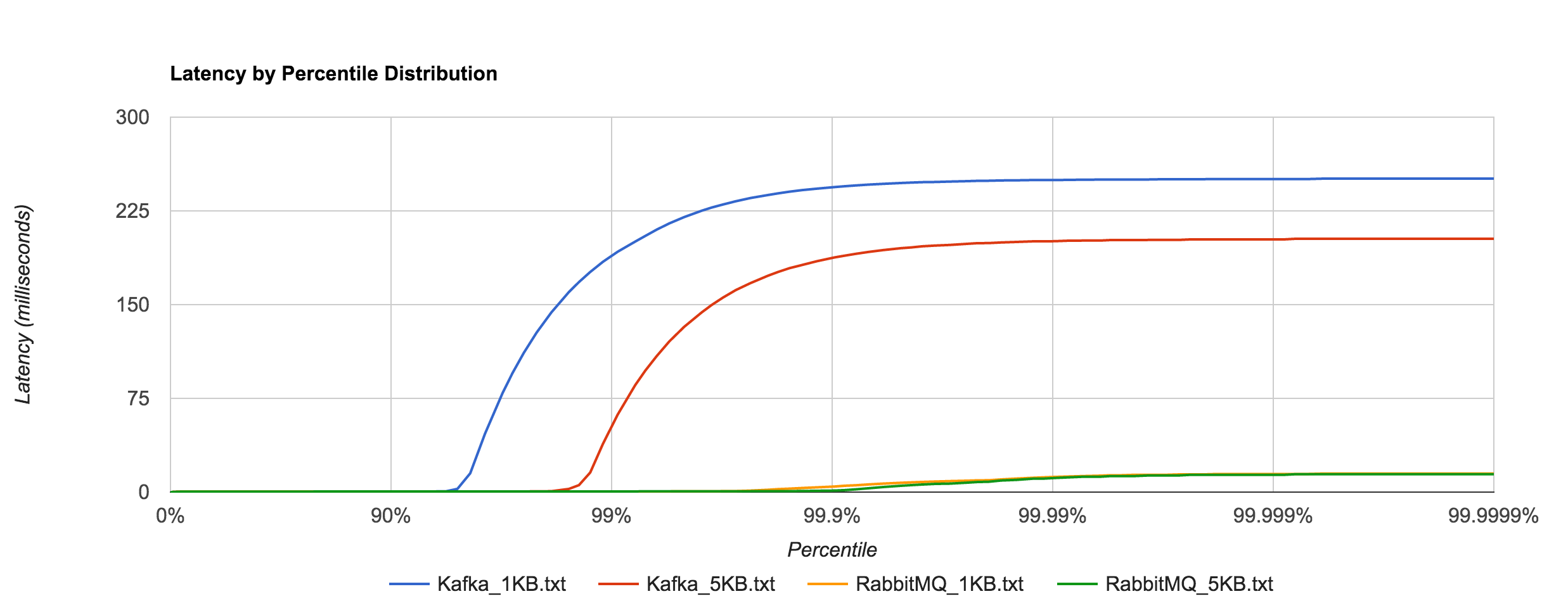
To show just how staggering the difference is, we can plot Kafka 0.8.2.2 and RabbitMQ 1MB latencies alongside Redis and NATS 5KB latencies. They are all within the same ballpark. Whatever the case may be, both RabbitMQ and Kafka appear to handle large messages extremely well in contrast to Redis and NATS.

This leads me to believe you’ll see better overall throughput, in terms of raw data, with RabbitMQ and Kafka, but more predictable, tighter tail latencies with Redis and NATS. Where SLAs are important, it’s hard to beat NATS. Of course, it’s unfair to compare Kafka with something like NATS or Redis or even RabbitMQ since they are very different (and sometimes complementary), but it’s also worth pointing out that the former is much more operationally complex.

However, benchmarking Kafka 0.9.0.0 (blue and red) shows an astounding difference in tail latencies compared to 0.8.2.2 (orange and green).

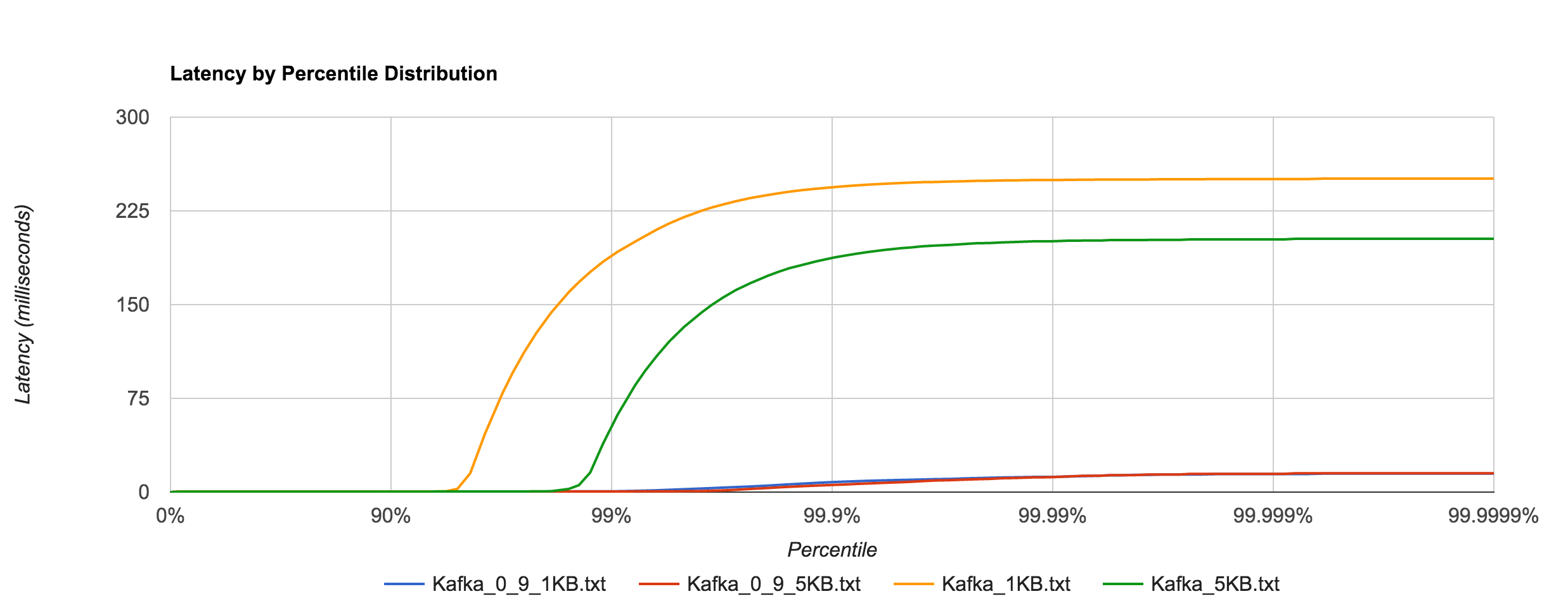
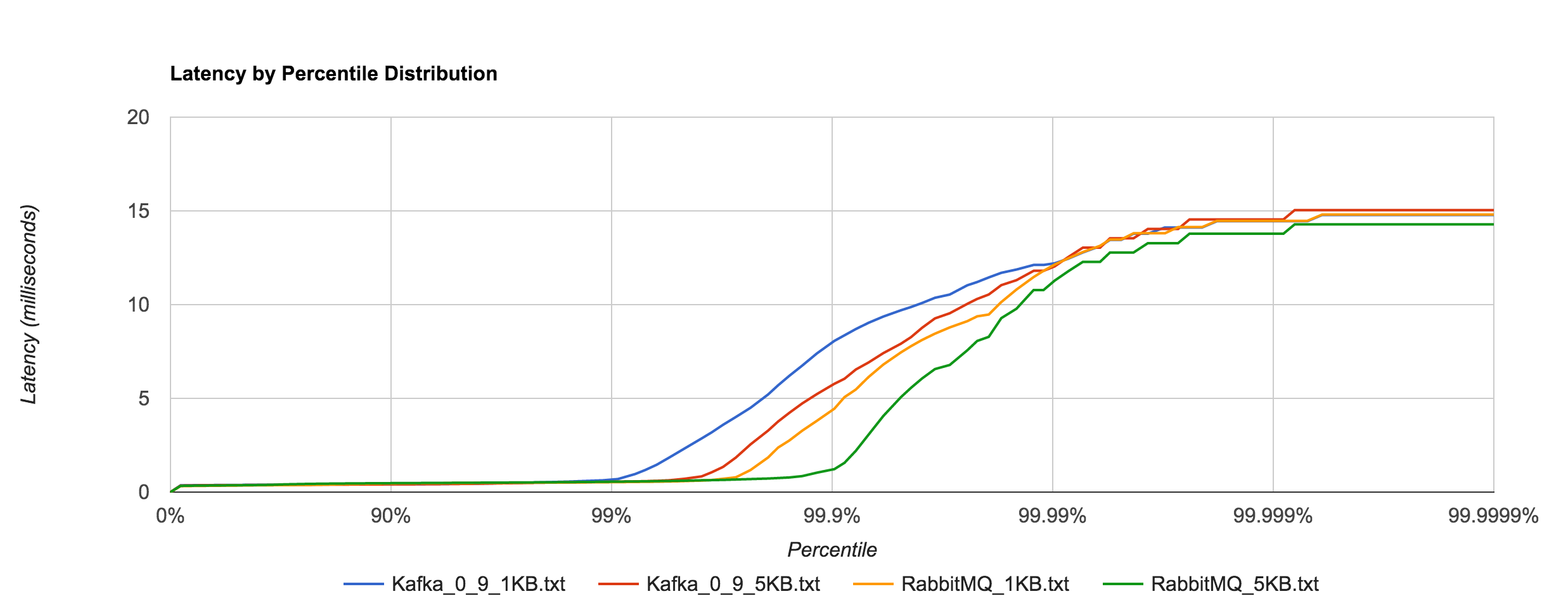
Kafka 0.9’s performance is much more in line with RabbitMQ’s at high percentiles as seen below.

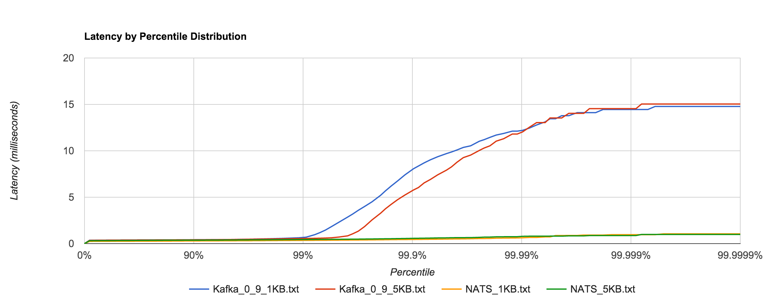
Likewise, it’s a much closer comparison to NATS when looking at the 1KB and 5KB runs.

As with 0.8, Kafka 0.9 does an impressive job dealing with 1MB messages in comparison to NATS, especially when looking at the 92nd percentile and beyond. It’s hard to decipher in the graph below, but Kafka 0.9’s 99th, 99.9th, and 99.99th percentile latencies are 0.66, 0.78, and 1.35 ms, respectively.

My initial thought was that the difference between Kafka 0.8 and 0.9 was attributed to a change in fsync behavior. To quote the Kafka documentation:

Kafka always immediately writes all data to the filesystem and supports the ability to configure the flush policy that controls when data is forced out of the OS cache and onto disk using the and flush. This flush policy can be controlled to force data to disk after a period of time or after a certain number of messages has been written.

However, there don’t appear to be any changes in the default flushing configuration between 0.8 and 0.9. The default configuration disables application fsync entirely, instead relying on the OS’s background flush. Jay Kreps indicates it’s a result of several “high percentile latency issues” that were fixed in 0.9. After scanning the 0.9 release notes, I was unable to determine specifically what those fixes might be. Either way, the difference is certainly not something to scoff at.

Conclusion

As always, interpret these benchmark results with a critical eye and perform your own tests if you’re evaluating these systems. This was more an exercise in benchmark methodology and tooling than an actual system analysis (and, as always, there’s still a lot of room for improvement). If anything, I think these results show how much we can miss by not looking beyond the 99th percentile. In almost all cases, everything looks pretty good up to that point, but after that things can get really bad. This is important to be conscious of when discussing SLAs.

I think the key takeaway is to consider your expected load in production, benchmark configurations around that, determine your allowable service levels, and iterate or provision more resources until you’re within those limits. The other important takeaway with respect to benchmarking is to look at the complete latency distribution. Otherwise, you’re not getting a clear picture of how your system actually behaves.

Follow @tyler_treat