Stream processing and related abstractions have become all the rage following the rise of systems like Apache Kafka, Samza, and the Lambda architecture. Applying the idea of immutable, append-only event sourcing means we’re storing more data than ever before. However, as the cost of storage continues to decline, it’s becoming more feasible to store more data for longer periods of time. With immutability, how the data lives isn’t interesting anymore. It’s all about how it moves.
The shifting landscape of data architecture parallels the way we’re designing systems today. Specifically, the evolution of monolithic to service-oriented architecture necessitates a change in the way we do data integration. The traditional normalization approach doesn’t cut it. Our systems are composed of databases, caches, search indexes, data warehouses, and a multitude of other components. Moreover, there’s an increasing demand for online, real-time processing of this data that’s tantamount to the growing popularity of large-scale, offline processing along the lines of Hadoop. This presents an interesting set of new challenges, namely, how do we drink from the firehose without getting drenched?
The answer most likely lies in frameworks like Samza, Storm, and Spark Streaming. Similarly, tools like StatsD solve the problem of collecting real-time analytics. However, this discussion is meant to explore some of the primitives used in stream processing. The ideas extend far beyond event sourcing, generalizing to any type of data stream, unbounded or not.
Batch vs. Streaming
With offline or batch processing, we often have some heuristics which provide insight into our data set, and we can typically afford multiple passes of the data. Without a strict time constraint, data structures are less important. We can store the entire data set on disk (or perhaps across a distributed file system) and process it in batches.
With streaming data, however, there’s a need for near real-time processing—collecting analytics, monitoring and alerting, updating search indexes and caches, etc. With web crawlers, we process a stream of URLs and documents and produce indexed content. With websites, we process a stream of page views and update various counters and gauges. With email, we process a stream of text and produce a filtered, spam-free inbox. These cases involve massive, often limitless data sets. Processing that data online can’t be done with the conventional ETL or MapReduce-style methods, and unless you’re doing windowed processing, it’s entirely impractical to store that data in memory.
Framing the Problem
As a concrete example of stream processing, imagine we want to count the number of distinct document views across a large corpus, say, Wikipedia. A naive solution would be to use a hash table which maps a document to a count. Wikipedia has roughly 35 million pages. Let’s assume each document is identified by a 16-byte GUID, and the counters are stored as 8-byte integers. This means we need in the ball park of a gigabyte of memory. Given today’s hardware, this might not sound completely unreasonable, but now let’s say we want to track views per unique IP address. We see that this approach quickly becomes intractable.
To illustrate further, consider how to count the cardinality of IP addresses which access our website. Instead of a hash table, we can use a bitmap or sparse bit array to count addresses. There are over four billion possible distinct IPv4 addresses. Sure, we could allocate half a gigabyte of RAM, but if you’re developing performance-critical systems, large heap sizes are going to kill you, and this overhead doesn’t help. ((Granted, if you’re sensitive to garbage-collection pauses, you may be better off using something like C or Rust, but that’s not always the most practical option.))
A Probabilistic Approach
Instead, we turn to probabilistic ways of solving these problems. Probabilistic algorithms and data structures seem to be oft-overlooked, or maybe purposely ignored, by system designers despite the theory behind them having been around for a long time in many cases. The goal should be to move these from the world of academia to industry because they are immensely useful and widely neglected.
Probabilistic solutions trade space and performance for accuracy. While a loss in precision may be a cause for concern to some, the fact is with large data streams, we have to trade something off to get real-time insight. Much like the CAP theorem, we must choose between consistency (accuracy) and availability (online). With CAP, we can typically adjust the level in which that trade-off occurs. This space/performance-accuracy exchange behaves very much the same way.
The literature can get pretty dense, so let’s look at what some of these approaches are and the problems they solve in a way that’s (hopefully) understandable.
Bloom Filters
The Bloom filter is probably the most well-known and, conceptually, simplest probabilistic data structure. It also serves as a good foundation because there are a lot of twists you can put on it. The theory provides a kernel from which many other probabilistic solutions are derived, as we will see.
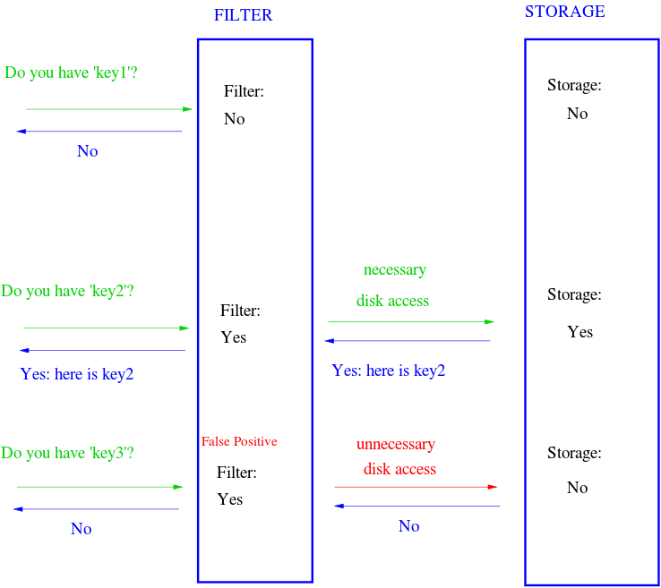
Bloom filters answer a simple question: is this element a member of a set? A normal set requires linear space because it stores every element. A Bloom filter doesn’t store the actual elements, it merely stores the “membership” of them. It uses sub-linear space opening the possibility for false positives, meaning there’s a non-zero probability it reports an item is in the set when it’s actually not. This has a wide range of applications. For example, a Bloom filter can be placed in front of a database. When a query for a piece of data comes in and the filter doesn’t contain it, we completely bypass the database.

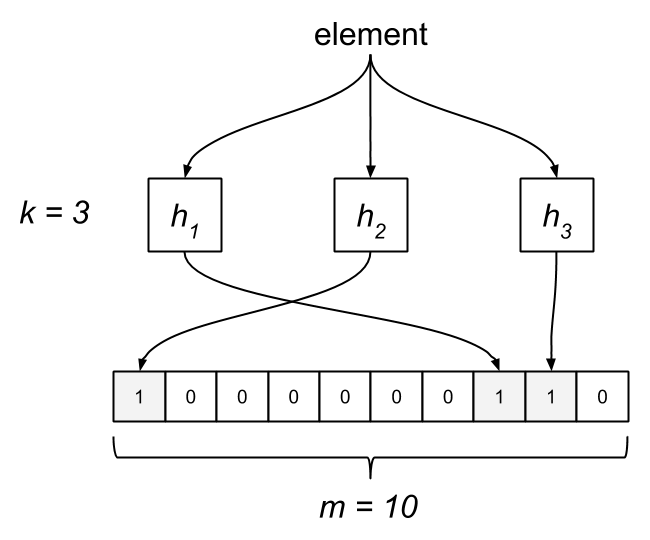
The Bloom filter consists of a bit array of length m and k hash functions. Both of these parameters are configurable, but we can optimize them based on a desired rate of false positives. Each bit in the array is initially unset. When an element is “added” to the filter, it’s hashed by each of the k functions, h1…hk, and modded by m, resulting in k indices into the bit array. Each bit at the respective index is set.

To query the membership of an element, we hash it and check if each bit is set. If any of them are zero, we know the item isn’t in the set. What happens when two different elements hash to the same index? This is where false positives are introduced. If the bits aren’t set, we know the element wasn’t added, but if they are, it’s possible that some other element or group of elements hashed to the same indices. Bloom filters have false positives, but false negatives are impossible—a member will never be reported incorrectly as a non-member. Unfortunately, this also means items can’t be removed from the filter.
It’s clear that the likelihood of false positives increases with each element added to the filter. We can target a specific probability of false positives by selecting an optimal value for m and k for up to n insertions. ((The math behind determining optimal m and k is left as an exercise for the reader.)) While this implementation works well in practice, it has a drawback in that some elements are potentially more sensitive to false positives than others. We can solve this problem by partitioning the m bits among the k hash functions such that each one produces an index over its respective partition. As a result, each element is always described by exactly k bits. This prevents any one element from being especially sensitive to false positives. Since calculating k hashes for every element is computationally expensive, we can actually perform a single hash and derive k hashes from it for a significant speedup. ((Less Hashing, Same Performance: Building a Better Bloom Filter discusses the use of two hash functions to simulate additional hashes. We can use a 64-bit hash, such as FNV, and use the upper and lower 32-bits as two different hashes.))
A Bloom filter eventually reaches a point where all bits are set, which means every query will indicate membership, effectively making the probability of false positives one. The problem with this is it requires a priori knowledge of the data set in order to select optimal parameters and avoid “overfilling.” Consequently, Bloom filters are ideal for offline processing and not so great for dealing with streams. Next, we’ll look at some variations of the Bloom filter which attempt to deal with this issue.
Scalable Bloom Filter
As we saw earlier, traditional Bloom filters are a great way to deal with set-membership problems in a space-efficient way, but they require knowing the size of the data set ahead of time in order to be effective. The Scalable Bloom Filter (SBF) was introduced by Almeida et al. as a way to cope with the capacity dilemma.
The Scalable Bloom Filter dynamically adapts to the size of the data set while enforcing a tight upper bound on the rate of false positives. Like the classic Bloom filter, false negatives are impossible. The SBF is essentially an array of Bloom filters with geometrically decreasing false-positive rates. New elements are added to the last filter. When this filter becomes “full”—more specifically, when it reaches a target fill ratio—a new filter is added with a tightened error probability. A tightening ratio, r, controls the growth of new filters.

Testing membership of an element consists of checking each of the filters. The geometrically decreasing false-positive rate of each filter is an interesting property. Since the fill ratio determines when a new filter is added, it turns out this progression can be modeled as a Taylor series which allows us to provide a tight upper bound on false positives using an optimal fill ratio of 0.5 (once the filter is 50% full, a new one is added). The compounded probability over the whole series converges to a target value, even accounting for an infinite series.
We can limit the error rate, but obviously the trade-off is that we end up allocating memory proportional to the size of the data set since we’re continuously adding filters. We also pay some computational cost on adds. Amortized, the cost of filter insertions is negligible, but for every add we must compute the current fill ratio of the filter to determine if a new filter needs to be added. Fortunately, we can optimize this by computing an estimated fill ratio. If we keep a running count of the items added to the filter, n, the approximate current fill ratio, p, can be obtained from the Taylor series expansion with  where m is the number of bits in the filter. Calculating this estimate turns out to be quite a bit faster than computing the actual fill ratio—fewer memory reads.
To provide some context around performance, adds in my Go implementation of a classic Bloom filter take about 166 ns on my MacBook Pro, and membership tests take 118 ns. With the SBF, adds take 422 ns and tests 113 ns. This isn’t a completely fair comparison since, as the SBF grows over time, tests require scanning through each filter, but certainly the add numbers are intuitive.
Scalable Bloom Filters are useful for cases where the size of the data set isn’t known a priori and memory constraints aren’t of particular concern. It’s an effective variation of a regular Bloom filter which generally requires space allocation orders-of-magnitude larger than the data set to allow enough headroom.
Stable Bloom Filter
Classic Bloom filters aren’t great for streaming data, and Scalable Bloom Filters, while a better option, still present a memory problem. Another derivative, the Stable Bloom Filter (SBF), was proposed by Deng and Rafiei as a technique for detecting duplicates in unbounded data streams with limited space. Most solutions work by dividing the stream into fixed-size windows and solving the problem within that discrete space. This allows the use of traditional methods like the Bloom filter.
The SBF attempts to approximate duplicates without the use of windows. Clearly, we can’t store the entire history of an infinite stream in limited memory. Instead, the thinking is more recent data has more value than stale data in many scenarios. As an example, web crawlers may not care about redundantly fetching a web page that was crawled a long time ago compared to fetching a page that was crawled more recently. With this impetus, the SBF works by representing more recent data while discarding old information.
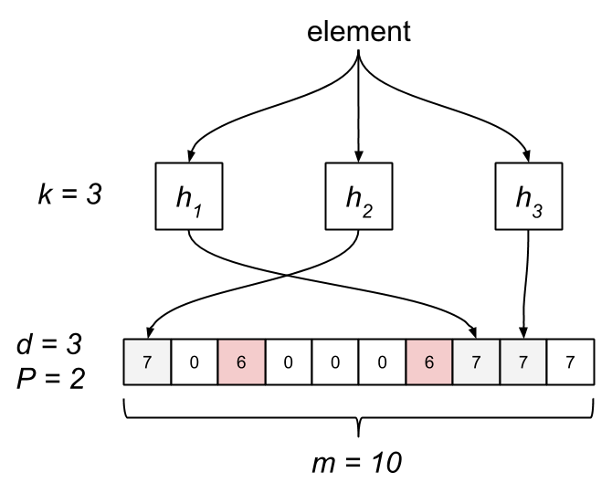
The Stable Bloom Filter tweaks the classic Bloom filter by replacing the bit array with an array of m cells, each allocated d bits. The cells are simply counters, initially set to zero. The maximum value, Max, of a cell is  . When an element is added, we first have to ensure space for it. This is done by selecting P random cells and decrementing their counters by one, clamping to zero. Next, we hash the element to k cells and set their counters to Max. Testing membership consists of probing the k cells. If any of them are zero, it’s not a member. The Bloom filter is actually a special case of an SBF where d is one and P is zero.

Like traditional Bloom filters, an SBF has a non-zero probability of false positives, which is controlled by several parameters. Unlike the Bloom filter, an SBF has a tight upper bound on the rate of false positives while introducing a non-zero rate of false negatives. The false-positive rate of a classic Bloom filter eventually reaches one, after which all queries result in a false positive. The stable-point property of an SBF means the false-positive rate asymptotically approaches a configurable fixed constant.
Stable Bloom Filters lend themselves to situations where the size of the data set isn’t known ahead of time and memory is bounded. For example, an SBF can be used to deduplicate events from an unbounded event stream with a specified upper bound on false positives and minimal false negatives. In particular, if the stream is not uniformly distributed, meaning duplicates are likely to be grouped closer together, the rate of false positives becomes immaterial.
Counting Bloom Filter
Conventional Bloom filters don’t allow items to be removed. The Stable Bloom Filter, on the other hand, works by evicting old data, but its API doesn’t expose a way to remove specific elements. The Counting Bloom Filter (CBF) is yet another twist on this structure. Introduced by Fan et al. in Summary Cache: A Scalable Wide-Area Web Cache Sharing Protocol, the CBF provides a way of deleting data from a filter.
It’s actually a very straightforward approach. The filter comprises an array of n-bit buckets similar to the Stable Bloom Filter. When an item is added, the corresponding counters are incremented, and when it’s removed, the counters are decremented.
Obviously, a CBF takes n-times more space than a regular Bloom filter, but it also has a scalability limit. Unless items are removed frequently enough, a counting filter’s false-positive probability will approach one. We need to dimension it accordingly, and this normally requires inferring from our data set. Likewise, since the CBF allows removals, it exposes an opportunity for false negatives. The multi-bit counters diminish the rate, but it’s important to be cognizant of this property so the CBF can be applied appropriately.
Inverse Bloom Filter
One of the distinguishing features of Bloom filters is the guarantee of no false negatives. This can be a valuable invariant, but what if we want the opposite of that? Is there an efficient data structure that can offer us no false positives with the possibility of false negatives? The answer is deceptively simple.
Jeff Hodges describes a rather trivial—yet strikingly pragmatic—approach which he calls the “opposite of a Bloom filter.” Since that name is a bit of a mouthful, I’m referring to this as the Inverse Bloom Filter (IBF).
The Inverse Bloom Filter may report a false negative but can never report a false positive. That is, it may indicate that an item has not been seen when it actually has, but it will never report an item as seen which it hasn’t come across. The IBF behaves in a similar manner to a fixed-size hash map of m buckets which doesn’t handle conflicts, but it provides lock-free concurrency using an underlying CAS.
The test-and-add operation hashes an element to an index in the filter. We take the value at that index while atomically storing the new value, then the old value is compared to the new one. If they differ, the new value wasn’t a member. If the values are equivalent, it was in the set.

The Inverse Bloom Filter is a nice option for dealing with unbounded streams or large data sets due to its limited memory usage. If duplicates are close together, the rate of false negatives becomes vanishingly small with an adequately sized filter.
HyperLogLog
Let’s revisit the problem of counting distinct IP addresses visiting a website. One solution might be to allocate a sparse bit array proportional to the number of IPv4 addresses. Alternatively, we could combine a Bloom filter with a counter. When an address comes in and it’s not in the filter, increment the count. While these both work, they’re not likely to scale very well. Rather, we can apply a probabilistic data structure known as the HyperLogLog (HLL). First presented by Flajolet et al. in 2007, HyperLogLog is an algorithm which approximately counts the number of distinct elements, or cardinality, of a multiset (a set which allows multiple occurrences of its elements).
Imagine our stream as a series of coin tosses. Someone tells you the most heads they flipped in a row was three. You can guess that they didn’t flip the coin very many times. However, if they flipped 20 heads in a row, it probably took them quite a while. This seems like a really unconvincing way of estimating the number of tosses, but from this kernel of thought grows a fruitful idea.
HLL replaces heads and tails with zeros and ones. Instead of counting the longest run of heads, it counts the longest run of leading zeros in a binary hash. Using a good hash function means that the values are, more or less, statistically independent and uniformly distributed. If the maximum run of leading zeros is n, the number of distinct elements in the set is approximately  . But wait, what’s the math behind this? If we think about it, half of all binary numbers start with 1. Each additional bit divides the probability of a run further in half; that is, 25% start with 01, 12.5% start with 001, 6.25% start with 0001, ad infinitum. Thus, the probability of a run of length n is
  .
.
Like flipping a coin, there’s potential for an enormous amount of variance with this technique. For instance, it’s entirely possible—though unlikely—that you flip 20 heads in a row on your first try. One experiment doesn’t provide enough data, so instead you flip 10 coins. HyperLogLog uses a similar strategy to reduce variance by splitting the stream up across a set of buckets, or registers, and applying the counting algorithm on the values in each one. It tracks the longest run of zeros in every register, and the total cardinality is computed by taking the harmonic mean across all registers. The harmonic mean is used to discount outliers since the distribution of values tends to skew towards the right. We can increase accuracy by adding more registers, which of course comes at the expense of performance and memory.
HyperLogLog is a remarkable algorithm. It almost feels like magic, and it’s exceptionally useful for working with data streams. HLL has a fraction of the memory footprint of other solutions. In fact, it’s usually several orders of magnitude while remaining surprisingly accurate.
Count-Min Sketch
HyperLogLog is a great option to efficiently count the number of distinct elements in a stream using a minimal amount of space, but it only gives us cardinality. What about counting the frequencies of specific elements? Cormode and Muthukrishnan developed the Count-Min sketch (CM sketch) to approximate the occurrences of different event types from a stream of events.
In contrast to a hash table, the Count-Min sketch uses sub-linear space to count frequencies. It consists of a matrix with w columns and d rows. These parameters determine the trade-off between space/time constraints and accuracy. Each row has an associated hash function. When an element arrives, it’s hashed for each row. The corresponding index in the rows are incremented by one. In this regard, the CM sketch shares some similarities with the Bloom filter.

The frequency of an element is estimated by taking the minimum of all the element’s respective counter values. The thought process here is that there is possibility for collisions between elements, which affects the counters for multiple items. Taking the minimum count results in a closer approximation.
The Count-Min sketch is an excellent tool for counting problems for the same reasons as HyperLogLog. It has a lot of similarities to Bloom filters, but where Bloom filters effectively represent sets, the CM sketch considers multisets.
MinHash
The last probabilistic technique we’ll briefly look at is MinHash. This algorithm, invented by Andrei Broder, is used to quickly estimate the similarity between two sets. This has a variety of uses, such as detecting duplicate bodies of text and clustering or comparing documents.
MinHash works, in part, by using the Jaccard coefficient, a statistic which represents the size of the intersection of two sets divided by the size of the union:

This provides a measure of how similar the two sets are, but computing the intersection and union is expensive. Instead, MinHash essentially works by comparing randomly selected subsets through element hashing. It resembles locality-sensitive hashing (LSH), which means that similar items have a greater tendency to map to the same hash values. This varies from most hashing schemes, which attempt to avoid collisions. Instead, LSH is designed to maximize collisions of similar elements.
MinHash is one of the more difficult algorithms to fully grasp, and I can’t even begin to provide a proper explanation. If you’re interested in how it works, read the literature but know that there are a number of variations of it. The important thing is to know it exists and what problems it can be applied to.
In Practice
We’ve gone over several fundamental primitives for processing large data sets and streams while solving a few different types of problems. Bloom filters can be used to reduce disk reads and other expensive operations. They can also be purposed to detect duplicate events in a stream or prune a large decision tree. HyperLogLog excels at counting the number of distinct items in a stream while using minimal space, and the Count-Min sketch tracks the frequency of particular elements. Lastly, the MinHash method provides an efficient mechanism for comparing the similarity between documents. This has a number of applications, namely around identifying duplicates and characterizing content.
While there are no doubt countless implementations for most of these data structures and algorithms, I’ve been putting together a Go library geared towards providing efficient techniques for stream processing called Boom Filters. It includes implementations for all of the probabilistic data structures outlined above. As streaming data and real-time consumption grow more and more prominent, it will become important that we have the tools and understanding to deal with them. If nothing else, it’s valuable to be aware of probabilistic methods because they often provide accurate results at a fraction of the cost. These things aren’t just academic research, they form the basis for building online, high-performance systems at scale.
