I originally proposed this as a GopherCon talk on writing “high-performance Go”, which is why it may seem rambling, incoherent, and—at times—not at all related to Go. The talk was rejected (probably because of the rambling and incoherence), but I still think it’s a subject worth exploring. The good news is, since it was rejected, I can take this where I want. The remainder of this piece is mostly the outline of that talk with some parts filled in, some meandering stories which may or may not pertain to the topic, and some lessons learned along the way. I think it might make a good talk one day, but this will have to do for now.
We work on some interesting things at Workiva—graph traversal, distributed and in-memory calculation engines, low-latency messaging systems, databases optimized for two-dimensional data computation. It turns out, when you want to build a complicated financial-reporting suite with the simplicity and speed of Microsoft Office, and put it entirely in the cloud, you can’t really just plumb some crap together and call it good. It also turns out that when you try to do this, performance becomes kind of important, not because of the complexity of the data—after all, it’s mostly just numbers and formulas—but because of the scale of it. Now, distribute that data in the cloud, consider the security and compliance implications associated with it, add in some collaboration and control mechanisms, and you’ve got yourself some pretty monumental engineering problems.
As I hinted at, performance starts to be really important, whether it’s performing a formula evaluation, publishing a data-change event, or opening up a workbook containing a million rows of data (accountants are weird). A lot of the backend systems powering all of this are, for better or worse, written in Go. Go is, of course, a garbage-collected language, and it compares closely to Java (though the latter has over 20 years invested in it, while the former has about seven).
At this point, you might be asking, “why not C?” It’s honestly a good question to ask, but the reality is there is always history. The first solution was written in Python on Google App Engine (something about MVPs, setting your customers’ expectations low, and giving yourself room to improve?). This was before Go was even a thing, though Java and C were definitely things, but this was a startup. And it was Python. And it was on App Engine. I don’t know exactly what led to those combination of things—I wasn’t there—but, truthfully, App Engine probably played a large role in the company’s early success. Python and App Engine were fast. Not like “this code is fucking fast” fast—what we call performance—more like “we need to get this shit working so we have jobs tomorrow” fast—what we call delivery. I don’t envy that kind of fast, but when you’re a startup trying to disrupt, speed to market matters a hell of a lot more than the speed of your software.
I’ve talked about App Engine at length before. Ultimately, you hit the ceiling of what you can do with it, and you have to migrate off (if you’re a business that is trying to grow, anyway). We hit that migration point at a really weird, uncomfortable time. This was right when Docker was starting to become a thing, and microservices were this thing that everybody was talking about but nobody was doing. Google had been successfully using containers for years, and Netflix was all about microservices. Everybody wanted to be like them, but no one really knew how—but it was the future (unikernels are the new future, by the way).
The problem is—coming from a PaaS like App Engine that does your own laundry—you don’t have the tools, skills, or experience needed to hit the ground running, so you kind of drunkenly stumble your way there. You don’t even have a DevOps team because you didn’t need one! Nobody knew how to use Docker, which is why at the first Dockercon, five people got on stage and presented five solutions to the same problem. It was the blind leading the blind. I love this article by Jesper L. Andersen, How to build stable systems, which contains a treasure trove of practical engineering tips. The very last paragraph of the article reads:
Docker is not mature (Feb 2016). Avoid it in production for now until it matures. Currently Docker is a time sink not fulfilling its promises. This will change over time, so know when to adopt it.
Trying to build microservices using Docker while everyone is stumbling over themselves was, and continues to be, a painful process, exacerbated by the heavy weight suddenly lifted by leaving App Engine. It’s not great if you want to go fast. App Engine made scaling easy by restricting you in what you could do, but once that burden was removed, it was off to the races. What people might not have realized, however, was that App Engine also made distributed systems easy by restricting you in what you could do. Some seem to think the limitations enforced by App Engine are there to make their lives harder or make Google richer (trust me, they’d bill you more if they could), so why would we have similar limitations in our own infrastructure? App Engine makes these limitations, of course, so that it can actually scale. Don’t take that for granted.
App Engine was stateless, so the natural tendency once you’re off it was to make everything stateful. And we did. What I don’t think we realized was that we were, in effect, trading one type of fast for the other—performance for delivery. We can build software that’s fast and runs on your desktop PC like in the 90’s, but now you want to put that in the cloud and make it scale? It takes a big infrastructure investment. It also takes a big time investment. Neither of which are good if you want to go fast, especially when you’re using enough microservices, Docker, and Go to rattle the Hacker News fart chamber. You kind of get caught in this endless rut of innovation that you almost lose your balance. Leaving the statelessness of App Engine for more stateful pastures was sort of like an infant learning to walk. You look down and it dawns on you—you have legs! So you run with it, because that’s amazing, and you stumble spectacularly a few times along the way. Finally, you realize maybe running full speed isn’t the best idea for someone who just learned to walk.
We were also making this transition while Go had started reaching critical mass. Every other headline in the tech aggregators was “why we switched to Go and you should too.” And we did. I swear this post has a point.
Tips for Writing High-Performance Go
By now, I’ve forgotten what I was writing about, but I promised this post was about Go. It is, and it’s largely about performance fast, not delivery fast—the two are often at odds with each other. Everything up until this point was mostly just useless context and ranting. But it also shows you that we are solving some hard problems and why we are where we are. There is always history.
I work with a lot of smart people. Many of us have a near obsession with performance, but the point I was attempting to make earlier is we’re trying to push the boundaries of what you can expect from cloud software. App Engine had some rigid boundaries, so we made a change. Since adopting Go, we’ve learned a lot about how to make things fast and how to make Go work in the world of systems programming.
Go’s simplicity and concurrency model make it an appealing choice for backend systems, but the larger question is how does it fare for latency-sensitive applications? Is it worth sacrificing the simplicity of the language to make it faster? Let’s walk through a few areas of performance optimization in Go—namely language features, memory management, and concurrency—and try to make that determination. All of the code for the benchmarks presented here are available on GitHub.
Channels
Channels in Go get a lot of attention because they are a convenient concurrency primitive, but it’s important to be aware of their performance implications. Usually the performance is “good enough” for most cases, but in certain latency-critical situations, they can pose a bottleneck. Channels are not magic. Under the hood, they are just doing locking. This works great in a single-threaded application where there is no lock contention, but in a multithreaded environment, performance significantly degrades. We can mimic a channel’s semantics quite easily using a lock-free ring buffer.
The first benchmark looks at the performance of a single-item-buffered channel and ring buffer with a single producer and single consumer. First, we look at the performance in the single-threaded case (GOMAXPROCS=1).
BenchmarkChannel 3000000 512 ns/op
BenchmarkRingBuffer 20000000 80.9 ns/op
As you can see, the ring buffer is roughly six times faster (if you’re unfamiliar with Go’s benchmarking tool, the first number next to the benchmark name indicates the number of times the benchmark was run before giving a stable result). Next, we look at the same benchmark with GOMAXPROCS=8.
BenchmarkChannel-8 3000000 542 ns/op
BenchmarkRingBuffer-8 10000000 182 ns/op
The ring buffer is almost three times faster.
Channels are often used to distribute work across a pool of workers. In this benchmark, we look at performance with high read contention on a buffered channel and ring buffer. The GOMAXPROCS=1 test shows how channels are decidedly better for single-threaded systems.
BenchmarkChannelReadContention 10000000 148 ns/op
BenchmarkRingBufferReadContention 10000 390195 ns/op
However, the ring buffer is faster in the multithreaded case:
BenchmarkChannelReadContention-8 1000000 3105 ns/op
BenchmarkRingBufferReadContention-8 3000000 411 ns/op
Lastly, we look at performance with contention on both the reader and writer. Again, the ring buffer’s performance is much worse in the single-threaded case but better in the multithreaded case.
BenchmarkChannelContention 10000 160892 ns/op
BenchmarkRingBufferContention 2 806834344 ns/op
BenchmarkChannelContention-8 5000 314428 ns/op
BenchmarkRingBufferContention-8 10000 182557 ns/op
The lock-free ring buffer achieves thread safety using only CAS operations. We can see that deciding to use it over the channel depends largely on the number of OS threads available to the program. For most systems, GOMAXPROCS > 1, so the lock-free ring buffer tends to be a better option when performance matters. Channels are a rather poor choice for performant access to shared state in a multithreaded system.
Defer
Defer is a useful language feature in Go for readability and avoiding bugs related to releasing resources. For example, when we open a file to read, we need to be careful to close it when we’re done. Without defer, we need to ensure the file is closed at each exit point of the function.
This is really error-prone since it’s easy to miss a return point. Defer solves this problem by effectively adding the cleanup code to the stack and invoking it when the enclosing function returns.
At first glance, one would think defer statements could be completely optimized away by the compiler. If I defer something at the beginning of a function, simply insert the closure at each point the function returns. However, it’s more complicated than this. For example, we can defer a call within a conditional statement or a loop. The first case might require the compiler to track the condition leading to the defer. The compiler would also need to be able to determine if a statement can panic since this is another exit point for a function. Statically proving this seems to be, at least on the surface, an undecidable problem.
The point is defer is not a zero-cost abstraction. We can benchmark it to show the performance overhead. In this benchmark, we compare locking a mutex and unlocking it with a defer in a loop to locking a mutex and unlocking it without defer.
BenchmarkMutexDeferUnlock-8 20000000 96.6 ns/op
BenchmarkMutexUnlock-8 100000000 19.5 ns/op
Using defer is almost five times slower in this test. To be fair, we’re looking at a difference of 77 nanoseconds, but in a tight loop on a critical path, this adds up. One trend you’ll notice with these optimizations is it’s usually up to the developer to make a trade-off between performance and readability. Optimization rarely comes free.
Reflection and JSON
Reflection is generally slow and should be avoided for latency-sensitive applications. JSON is a common data-interchange format, but Go’s encoding/json package relies on reflection to marshal and unmarshal structs. With ffjson, we can use code generation to avoid reflection and benchmark the difference.
BenchmarkJSONReflectionMarshal-8 200000 7063 ns/op
BenchmarkJSONMarshal-8 500000 3981 ns/op
BenchmarkJSONReflectionUnmarshal-8 200000 9362 ns/op
BenchmarkJSONUnmarshal-8 300000 5839 ns/op
Code-generated JSON is about 38% faster than the standard library’s reflection-based implementation. Of course, if we’re concerned about performance, we should really avoid JSON altogether. MessagePack is a better option with serialization code that can also be generated. In this benchmark, we use the msgp library and compare its performance to JSON.
BenchmarkMsgpackMarshal-8 3000000 555 ns/op
BenchmarkJSONReflectionMarshal-8 200000 7063 ns/op
BenchmarkJSONMarshal-8 500000 3981 ns/op
BenchmarkMsgpackUnmarshal-8 20000000 94.6 ns/op
BenchmarkJSONReflectionUnmarshal-8 200000 9362 ns/op
BenchmarkJSONUnmarshal-8 300000 5839 ns/op
The difference here is dramatic. Even when compared to the generated JSON serialization code, MessagePack is significantly faster.
If we’re really trying to micro-optimize, we should also be careful to avoid using interfaces, which have some overhead not just with marshaling but also method invocations. As with other kinds of dynamic dispatch, there is a cost of indirection when performing a lookup for the method call at runtime. The compiler is unable to inline these calls.
BenchmarkJSONReflectionUnmarshal-8 200000 9362 ns/op
BenchmarkJSONReflectionUnmarshalIface-8 200000 10099 ns/op
We can also look at the overhead of the invocation lookup, I2T, which converts an interface to its backing concrete type. This benchmark calls the same method on the same struct. The difference is the second one holds a reference to an interface which the struct implements.
BenchmarkStructMethodCall-8 2000000000 0.44 ns/op
BenchmarkIfaceMethodCall-8 1000000000 2.97 ns/op
Sorting is a more practical example that shows the performance difference. In this benchmark, we compare sorting a slice of 1,000,000 structs and 1,000,000 interfaces backed by the same struct. Sorting the structs is nearly 92% faster than sorting the interfaces.
BenchmarkSortStruct-8 10 105276994 ns/op
BenchmarkSortIface-8 5 286123558 ns/op
To summarize, avoid JSON if possible. If you need it, generate the marshaling and unmarshaling code. In general, it’s best to avoid code that relies on reflection and interfaces and instead write code that uses concrete types. Unfortunately, this often leads to a lot of duplicated code, so it’s best to abstract this with code generation. Once again, the trade-off manifests.
Memory Management
Go doesn’t actually expose heap or stack allocation directly to the user. In fact, the words “heap” and “stack” do not appear anywhere in the language specification. This means anything pertaining to the stack and heap are technically implementation-dependent. In practice, of course, Go does have a stack per goroutine and a heap. The compiler does escape analysis to determine if an object can live on the stack or needs to be allocated in the heap.
Unsurprisingly, avoiding heap allocations can be a major area of optimization. By allocating on the stack, we avoid expensive malloc calls, as the benchmark below shows.
BenchmarkAllocateHeap-8 20000000 62.3 ns/op 96 B/op 1 allocs/op
BenchmarkAllocateStack-8 100000000 11.6 ns/op 0 B/op 0 allocs/op
Naturally, passing by reference is faster than passing by value since the former requires copying only a pointer while the latter requires copying values. The difference is negligible with the struct used in these benchmarks, though it largely depends on what has to be copied. Keep in mind there are also likely some compiler optimizations being performed in this synthetic benchmark.
BenchmarkPassByReference-8 1000000000 2.35 ns/op
BenchmarkPassByValue-8 200000000 6.36 ns/op
However, the larger issue with heap allocation is garbage collection. If we’re creating lots of short-lived objects, we’ll cause the GC to thrash. Object pooling becomes quite important in these scenarios. In this benchmark, we compare allocating structs in 10 concurrent goroutines on the heap vs. using a sync.Pool for the same purpose. Pooling yields a 5x improvement.
BenchmarkConcurrentStructAllocate-8 5000000 337 ns/op
BenchmarkConcurrentStructPool-8 20000000 65.5 ns/op
It’s important to point out that Go’s sync.Pool is drained during garbage collection. The purpose of sync.Pool is to reuse memory between garbage collections. One can maintain their own free list of objects to hold onto memory across garbage collection cycles, though this arguably subverts the purpose of a garbage collector. Go’s pprof tool is extremely useful for profiling memory usage. Use it before blindly making memory optimizations.
False Sharing
When performance really matters, you have to start thinking at the hardware level. Formula One driver Jackie Stewart is famous for once saying, “You don’t have to be an engineer to be be a racing driver, but you do have to have mechanical sympathy.” Having a deep understanding of the inner workings of a car makes you a better driver. Likewise, having an understanding of how a computer actually works makes you a better programmer. For example, how is memory laid out? How do CPU caches work? How do hard disks work?
Memory bandwidth continues to be a limited resource in modern CPU architectures, so caching becomes extremely important to prevent performance bottlenecks. Modern multiprocessor CPUs cache data in small lines, typically 64 bytes in size, to avoid expensive trips to main memory. A write to a piece of memory will cause the CPU cache to evict that line to maintain cache coherency. A subsequent read on that address requires a refresh of the cache line. This is a phenomenon known as false sharing, and it’s especially problematic when multiple processors are accessing independent data in the same cache line.
Imagine a struct in Go and how it’s laid out in memory. Let’s use the ring buffer from earlier as an example. Here’s what that struct might normally look like:
The queue and dequeue fields are used to determine producer and consumer positions, respectively. These fields, which are both eight bytes in size, are concurrently accessed and modified by multiple threads to add and remove items from the queue. Since these two fields are positioned contiguously in memory and occupy only 16 bytes of memory, it’s likely they will stored in a single CPU cache line. Therefore, writing to one will result in evicting the other, meaning a subsequent read will stall. In more concrete terms, adding or removing things from the ring buffer will cause subsequent operations to be slower and will result in lots of thrashing of the CPU cache.
We can modify the struct by adding padding between fields. Each padding is the width of a single CPU cache line to guarantee the fields end up in different lines. What we end up with is the following:
How big a difference does padding out CPU cache lines actually make? As with anything, it depends. It depends on the amount of multiprocessing. It depends on the amount of contention. It depends on memory layout. There are many factors to consider, but we should always use data to back our decisions. We can benchmark operations on the ring buffer with and without padding to see what the difference is in practice.
First, we benchmark a single producer and single consumer, each running in a goroutine. With this test, the improvement between padded and unpadded is fairly small, about 15%.
BenchmarkRingBufferSPSC-8 10000000 156 ns/op
BenchmarkRingBufferPaddedSPSC-8 10000000 132 ns/op
However, when we have multiple producers and multiple consumers, say 100 each, the difference becomes slightly more pronounced. In this case, the padded version is about 36% faster.
BenchmarkRingBufferMPMC-8 100000 27763 ns/op
BenchmarkRingBufferPaddedMPMC-8 100000 17860 ns/op
False sharing is a very real problem. Depending on the amount of concurrency and memory contention, it can be worth introducing padding to help alleviate its effects. These numbers might seem negligible, but they start to add up, particularly in situations where every clock cycle counts.
Lock-Freedom
Lock-free data structures are important for fully utilizing multiple cores. Considering Go is targeted at highly concurrent use cases, it doesn’t offer much in the way of lock-freedom. The encouragement seems to be largely directed towards channels and, to a lesser extent, mutexes.
That said, the standard library does offer the usual low-level memory primitives with the atomic package. Compare-and-swap, atomic pointer access—it’s all there. However, use of the atomic package is heavily discouraged:
We generally don’t want sync/atomic to be used at all…Experience has shown us again and again that very very few people are capable of writing correct code that uses atomic operations…If we had thought of internal packages when we added the sync/atomic package, perhaps we would have used that. Now we can’t remove the package because of the Go 1 guarantee.
How hard can lock-free really be though? Just rub some CAS on it and call it a day, right? After a sufficient amount of hubris, I’ve come to learn that it’s definitely a double-edged sword. Lock-free code can get complicated in a hurry. The atomic and unsafe packages are not easy to use, at least not at first. The latter gets its name for a reason. Tread lightly—this is dangerous territory. Even more so, writing lock-free algorithms can be tricky and error-prone. Simple lock-free data structures, like the ring buffer, are pretty manageable, but anything more than that starts to get hairy.
The Ctrie, which I wrote about in detail, was my foray into the world of lock-free data structures beyond your standard fare of queues and lists. Though the theory is reasonably understandable, the implementation is thoroughly complex. In fact, the complexity largely stems from the lack of a native double compare-and-swap, which is needed to atomically compare indirection nodes (to detect mutations on the tree) and node generations (to detect snapshots taken of the tree). Since no hardware provides such an operation, it has to be simulated using standard primitives (and it can).
The first Ctrie implementation was actually horribly broken, and not even because I was using Go’s synchronization primitives incorrectly. Instead, I had made an incorrect assumption about the language. Each node in a Ctrie has a generation associated with it. When a snapshot is taken of the tree, its root node is copied to a new generation. As nodes in the tree are accessed, they are lazily copied to the new generation (à la persistent data structures), allowing for constant-time snapshotting. To avoid integer overflow, we use objects allocated on the heap to demarcate generations. In Go, this is done using an empty struct. In Java, two newly constructed Objects are not equivalent when compared since their memory addresses will be different. I made a blind assumption that the same was true in Go, when in fact, it’s not. Literally the last paragraph of the Go language specification reads:
A struct or array type has size zero if it contains no fields (or elements, respectively) that have a size greater than zero. Two distinct zero-size variables may have the same address in memory.
Oops. The result was that two different generations were considered equivalent, so the double compare-and-swap always succeeded. This allowed snapshots to potentially put the tree in an inconsistent state. That was a fun bug to track down. Debugging highly concurrent, lock-free code is hell. If you don’t get it right the first time, you’ll end up sinking a ton of time into fixing it, but only after some really subtle bugs crop up. And it’s unlikely you get it right the first time. You win this time, Ian Lance Taylor.
But wait! Obviously there’s some payoff with complicated lock-free algorithms or why else would one subject themselves to this? With the Ctrie, lookup performance is comparable to a synchronized map or a concurrent skip list. Inserts are more expensive due to the increased indirection. The real benefit of the Ctrie is its scalability in terms of memory consumption, which, unlike most hash tables, is always a function of the number of keys currently in the tree. The other advantage is its ability to perform constant-time, linearizable snapshots. We can compare performing a “snapshot” on a synchronized map concurrently in 100 different goroutines with the same test using a Ctrie:
BenchmarkConcurrentSnapshotMap-8 1000 9941784 ns/op
BenchmarkConcurrentSnapshotCtrie-8 20000 90412 ns/op
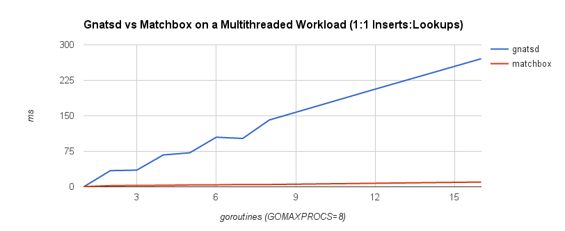
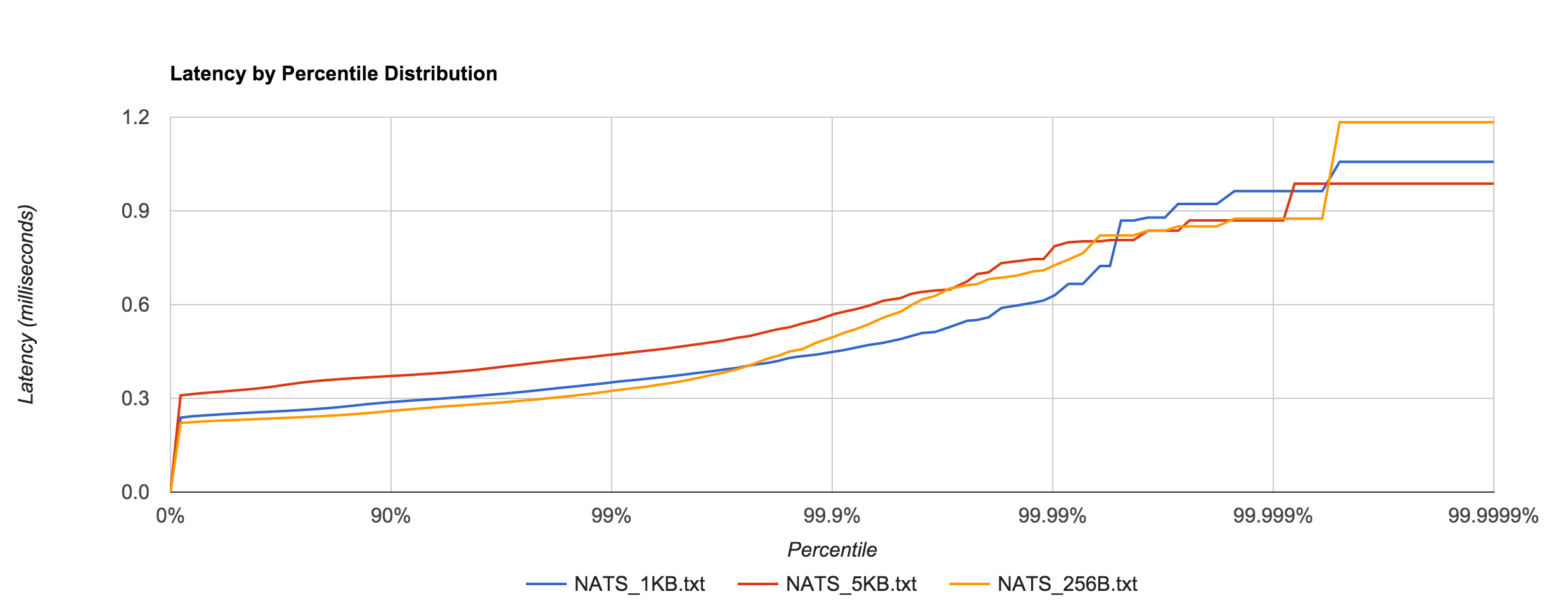
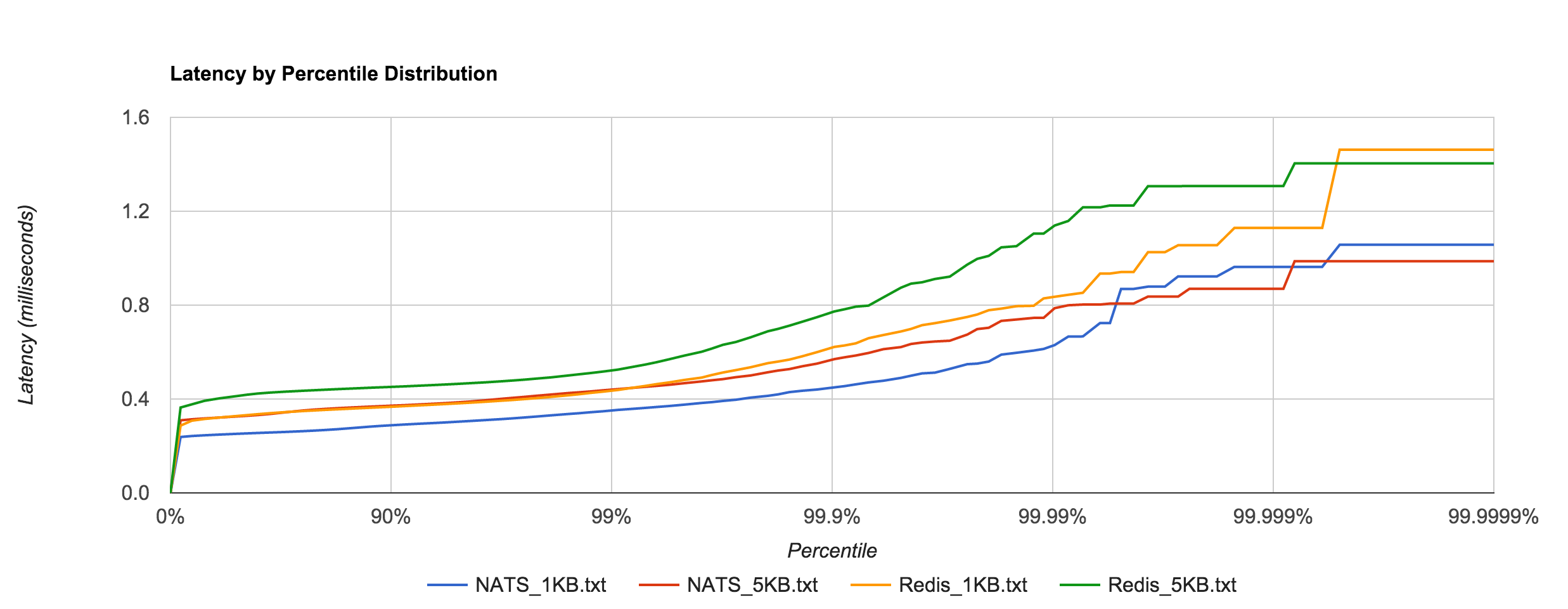
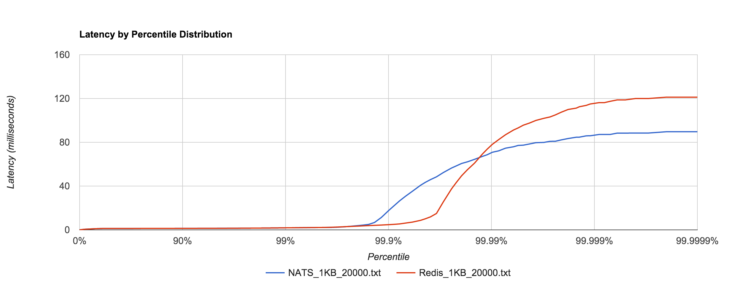
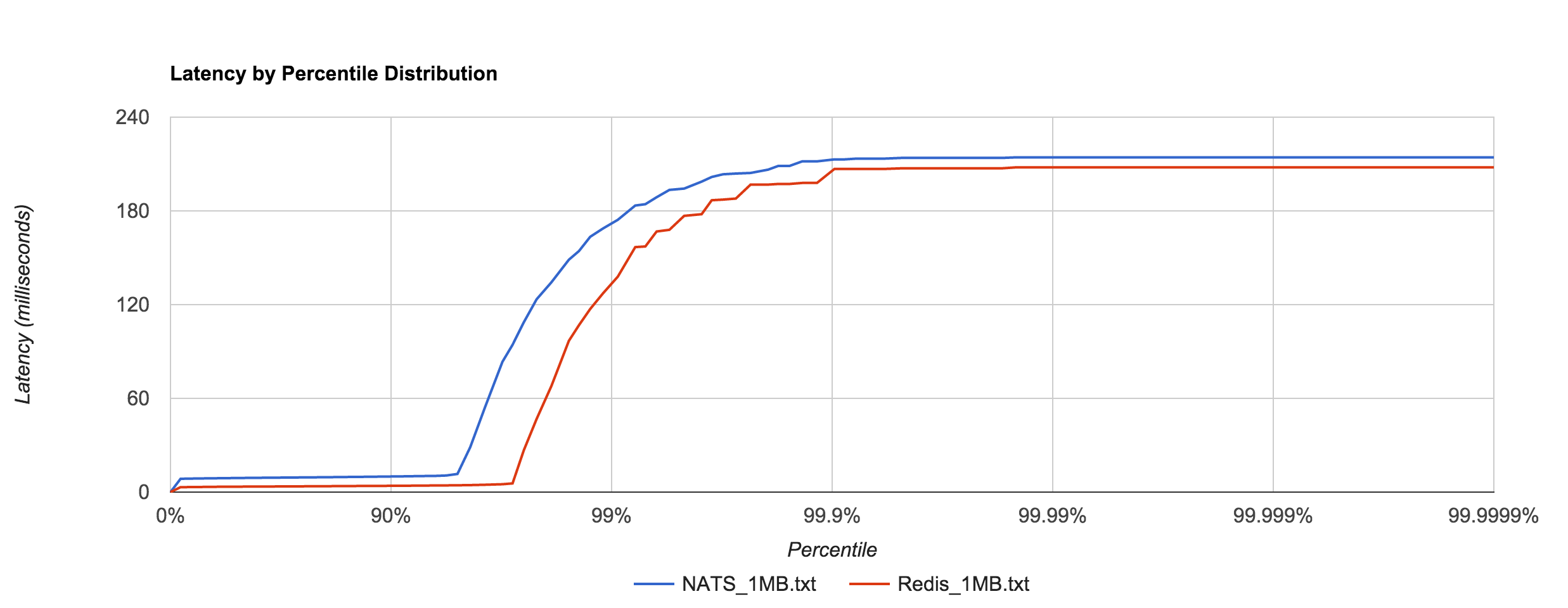
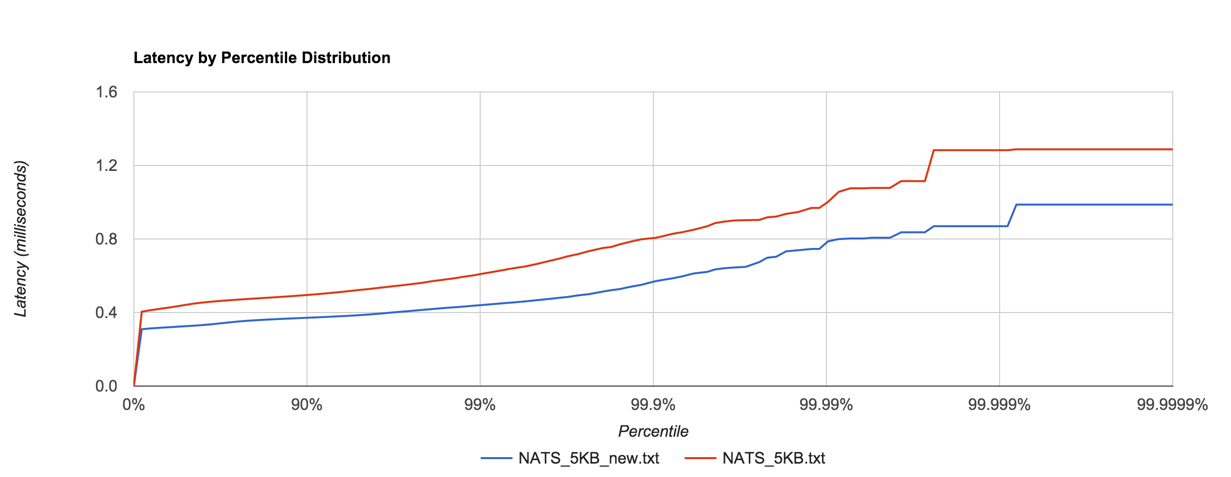
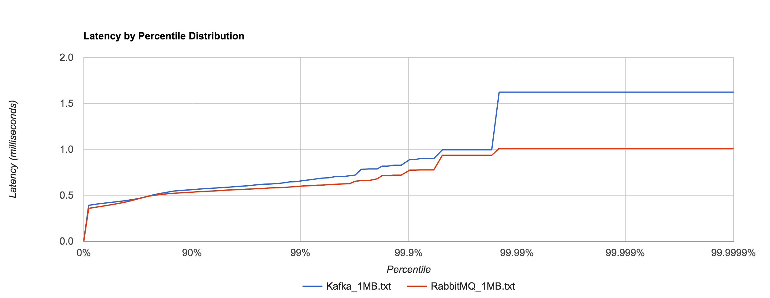
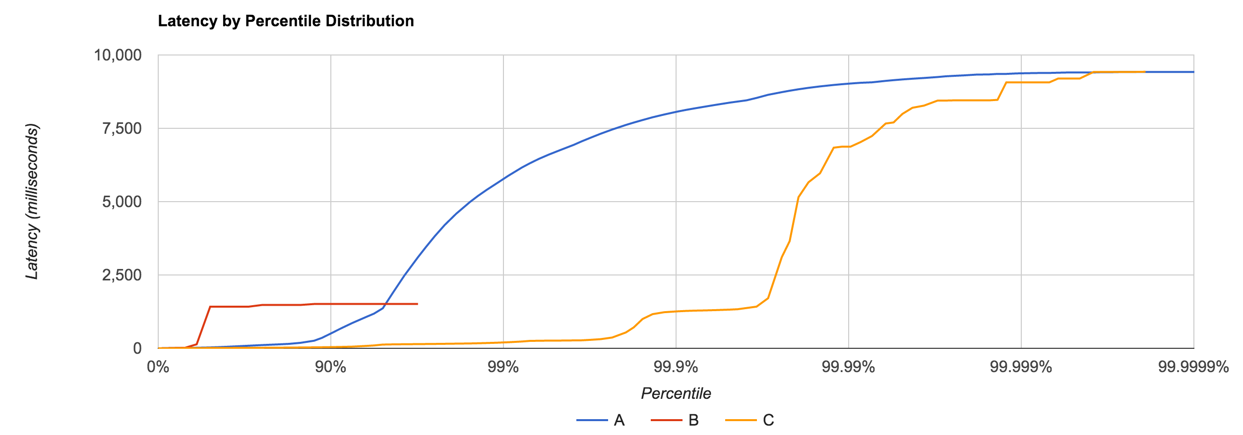
Depending on access patterns, lock-free data structures can offer better performance in multithreaded systems. For example, the NATS message bus uses a synchronized map-based structure to perform subscription matching. When compared with a Ctrie-inspired, lock-free structure, throughput scales a lot better. The blue line is the lock-based data structure, while the red line is the lock-free implementation.
Avoiding locks can be a boon depending on the situation. The advantage was apparent when comparing the ring buffer to the channel. Nonetheless, it’s important to weigh any benefit against the added complexity of the code. In fact, sometimes lock-freedom doesn’t provide any tangible benefit at all!
A Note on Optimization
As we’ve seen throughout this post, performance optimization almost always comes with a cost. Identifying and understanding optimizations themselves is just the first step. What’s more important is understanding when and where to apply them. The famous quote by C. A. R. Hoare, popularized by Donald Knuth, has become a longtime adage of programmers:
The real problem is that programmers have spent far too much time worrying about efficiency in the wrong places and at the wrong times; premature optimization is the root of all evil (or at least most of it) in programming.
Though the point of this quote is not to eliminate optimization altogether, it’s to learn how to strike a balance between speeds—speed of an algorithm, speed of delivery, speed of maintenance, speed of a system. It’s a highly subjective topic, and there is no single rule of thumb. Is premature optimization the root of all evil? Should I just make it work, then make it fast? Does it need to be fast at all? These are not binary decisions. For example, sometimes making it work then making it fast is impossible if there is a fundamental problem in the design.
However, I will say focus on optimizing along the critical path and outward from that only as necessary. The further you get from that critical path, the more likely your return on investment is to diminish and the more time you end up wasting. It’s important to identify what adequate performance is. Do not spend time going beyond that point. This is an area where data-driven decisions are key—be empirical, not impulsive. More important, be practical. There’s no use shaving nanoseconds off of an operation if it just doesn’t matter. There is more to going fast than fast code.
Wrapping Up
If you’ve made it this far, congratulations, there might be something wrong with you. We’ve learned that there are really two kinds of fast in software—delivery and performance. Customers want the first, developers want the second, and CTOs want both. The first is by far the most important, at least when you’re trying to go to market. The second is something you need to plan for and iterate on. Both are usually at odds with each other.
Perhaps more interestingly, we looked at a few ways we can eke out that extra bit of performance in Go and make it viable for low-latency systems. The language is designed to be simple, but that simplicity can sometimes come at a price. Like the trade-off between the two fasts, there is a similar trade-off between code lifecycle and code performance. Speed comes at the cost of simplicity, at the cost of development time, and at the cost of continued maintenance. Choose wisely.


